How Our Presidential Forecast Works
Breaking down our 2024 model, and what's changed now that it's a new matchup.
This is the full methodology post for our 2024 Presidential Forecast, found at the link below:
How to interpret the forecast
Before I go into more detail on how the model calculates and creates things, I want to establish how you should use it in practice. First, it is NOT a prediction. There is a huge grey area between using forecast, prediction, estimate, model, etc. when labeling a project like this. But my personal view is that a prediction is declaratory. If I am predicting whether or not there will be a snow day tomorrow, I am telling you that there will be one or not. A forecast, not unlike basic weather forecasts that we all use daily, offers a probabilistic view of the situation instead. In the case of the presidential election, a prediction would be me saying “I predict Trump will win”. But that’s just not useful. A forecast allows me to say “Trump is the slight favorite to win”, indicating that while he is more likely than not to do so, there is a certain amount of uncertainty. The odds themselves quantify that uncertainty.
So, when you look at the odds, don’t think of it as a sure thing that the leading candidate will win. (As of writing this post, it’s anything but a sure thing, with Trump only having a 52.6% chance.) Think of it as an indicator of how likely a win is for Trump and Harris. (This is why there is an upset analogy) Now, unlike weather forecasts, which model the chance of it as an entire area, meaning an 80% chance of rain implies each inch of the forecast area has an 80% chance of rain, or 80% of the area should see rain, elections are to win. There are differences with elections in that there are only two possible outcomes: A Trump win or a Harris win. The odds are based on 100,000 simulations of different scenarios. Only one of those scenarios will happen, and the best way to make an educated guess of what that scenario will be is through a forecast.
But it’s not Election Day. Won’t this change?
Yes. However, unlike the very basic nowcast that was on the site a month or so ago, the model is meant to simulate the election assuming it occurs on November 5th. It takes into account this gap in time in a few ways, which will be discussed in more detail below. But the nowcast had a moving target date, trying to simulate an election held today with each update, whereas this simulates it on November 5th each time. This means it’s actually “forecasting”, with emphasis on the “fore” meaning to predict before. I have considered posting the nowcast odds on the forecast page, but I don’t see a huge appeal to doing so, and it would require extra work with each update.
Biden dropped out. What changed in the model?
There are two different types of changes that were implemented when Biden ended his re-election bid; required changes to keep the model up to date on the candidates, or activating what Nate Silver calls “Kamala mode” and additional fixes and improvements that I added to take advantage of the break.
Biden —> Harris changes
Resetting polling averages: This was a painful one. I had to go into each of the (55?) state/district presidential averages, (which are now at HenryDRiley.com) change the labeling from Biden to Harris, delete all Biden-Trump polls, add in Harris-Trump polls conducted fully on or after July 21st, (the day Biden dropped out) and note the change on the charts.
Change labeling on the forecast page: Nothing to note here, I just replaced any references to Biden with Harris on the forecast you see.
Fill in all the new data into the averages and model.
Other changes
Polling average improvements: Two main changes here, one of which was already being implemented but is now fully in place. That’s the fact that I only include polls with third parties included, and polls with just Harris and Trump are adjusted to include support for others. This is done by simply taking the current third-party average, splitting it into two, and subtracting that from both Harris and Trump’s vote shares. The second change is that when survey results down to the tenth place are available, I don’t round within the average itself, therefore in theory making the average more precise and less subject to rounding bias. For example, a poll that is in reality 41.4% Harris and 42.6% Trump only has a 1.2% margin, but rounding would indicate a 2% lead, being over-confident. You will not see this change on the list of polls, as those lists are still rounded, but the unrounded version is used in the actual calculations and averages.
Home state adjustments: This one’s pretty simple, and it effectively just gives a small boost to both campaigns in their nominees (including VPs, so Harris will still get a boost later - more to come on this) home states. The formula below was created by looking at the historical average margin improvement in home states from various studies, and attempts to follow the historical trend that bigger states see smaller boosts, and vice versa. It should be noted that this boost is applied solely to the fundamental forecast, so a 1% boost only has at most a 0.4% impact on the overall model.
Presidential nominee margin boost in their home state: 0.5*(7)/(sqrt(electoral votes))
The Vice Presidential nominee margin boost in their home state is typically ¼ as large: 0.125*(7)/(sqrt(electoral votes))
Currently, the home state adjustments to the overall forecasts are:
Kamala Harris (California - 54 electoral votes) - +0.4% margin
Running mate - TBD
Donald Trump (Florida - 30 electoral votes) - +0.4% margin
J.D. Vance (Ohio - 17 electoral votes) - +0.2% margin
Maine & Nebraska fix: If you’ve ever looked into past presidential elections, you may notice that Maine and Nebraska work a bit differently than the other 48 states. That’s because while they both award two electoral votes to the statewide winner (called winner-take-all), the rest of their electoral votes (two for Maine and three for Nebraska) are split up and awarded to the winners of each congressional district. (of which there are, you guessed it, two for Maine, and three for Nebraska) This makes modeling these two states a bit tricky, because we often get a lot more statewide polling, particularly for Maine, than we do district-level polling. It also forces me to decide how to model the state best, and what data to use. The Biden-Trump model incorrectly simulated the statewide and congressional districts as completely separate states. This meant that in theory, Biden could lose both of Maine’s congressional districts and still win statewide in a given simulation. (That isn’t possible) Now, the model simply simulates each congressional district, ignoring statewide data, and then totals them up to get the statewide result.
Ok, how does it work?
Now let’s get onto the nitty-gritty of this post; how the model functions. I’m going to walk you through the gist of all the steps within the forecast, explaining as I go the role and functionality of each of the parts, all of which work together.
1. Polling averages
This is explained in detail at HenryDRiley.com/Polls
2. Create the base fundamentals projection using national polling and an economic adjustment
Here, we take the current national polling average and apply our economic adjustment to get a starting fundamentals projection for use in state forecasts later on. For the economic adjustment, we take into account the following consumer confidence surveys:
Each survey has its own numerical system in terms of what’s a “good” and “bad” outlook on the economy by consumers, based on historical values. We take into account those historical values to determine how the current reading deviates from what historically is considered “average”. For the UMich survey, a value between 70 & 90 is considered “normal” by our model, while anything below 70 hurts the incumbent (Harris) and anything above 90 helps her. Values in between do not affect the polling average. For the Conference Board survey, 100 is considered average, and 0 is considered average for the Gallup index.
Once we have the three adjustments from each of the surveys, we simply average them out to get our final economic adjustment. That final adjustment is then applied to the current national polling margin, so a 2% adjustment would boost Harris’s average by 1%, and lower Trump’s by 1%.
3. Create a fundamentals-based projection for each state
It’s important to clarify what I mean by a “fundamentals” vs “polling” estimate. When I’m referring to the “polling weight” or a “polls-only forecast”, that means it is solely using state polls. The fundamentals estimate still uses national polls as a starting point, and then tweaks each state to about where it should be compared to the national projection. Essentially, if the national average was Harris +1, and our fundamentals projection said Trump should be +20 in Alabama compared to the country, then he’d be +19 in Alabama.
To get this adjustment for each state, we start with a basic “state partisanship” adjustment, taking into account the following, with the order they are listed in is the order the model weighs them:
The Cook PVI (Partisan Voting Index), is essentially an average of the margin from the last two presidential elections in the state
The average margin from the last two Senate elections in the state
The average margin from the last two elections for Governor in the state
For Wisconsin, this adjustment is about D+1, so based on recent elections alone, Democrats should do about a point better than they do nationally.
The next adjustment is all about the money. We simply take the total individual contribution amounts (per the Federal Elections Commission), calculate those amounts as percentages, and then calculate the margin between those percentages. So if Harris has raised 52% of the total Harris & Trump contributions, then the margin would be 4%. (52-48) Using this margin alone to adjust our projection would be too large, though, as safe states like Washington would give Harris a 37% adjustment, which is insane. So we take the logarithm (base 10) of the margin instead, so the largest fundraising adjustment is only about 2% of the vote.
Finally, we adjust for President Biden’s approval rating in each state. Now you may be thinking, “He isn’t running anymore!”, but we believe that the approval rating of the incumbent is a metric that should apply to the incumbent party as a whole, and to be fair, the nominee is still the incumbent Vice President, and it is the Biden-Harris administration. We take Race to the WH’s forecasted net approval for each state and again take the base 10 logarithm of that net approval forecast as our approval adjustment.
Now that we have all of the separate adjustments hashed out, we simply add them all together and then apply that final adjustment to our (national) base fundamentals projection from step two. Then, we can adjust for undecideds to get a purely fundamentals-based projection of how the state will vote.
4. Create a polls-based projection for each state
The polling projections are relatively simple, but there are a few more complex steps involved here. The first thing the model does to create a polls-based vote share is simply input the current polling average for each state if one is available.
An adjustment that the model makes is that it effectively tries to “sync” state polling averages with the national average. If we haven’t had polls from Arizona in two weeks, the model will take the Arizona average and apply the national trends over that period to the state average to fill in the gap. This helps us get a more realistic polling picture, and the underlying theory is that if state results are heavily correlated to national results, almost 1:1, then national movement should roughly translate 1:1 with state movement too.
The final step is to simply adjust for undecided voters. Both Harris and Trump get 40% of any leftover undecideds, and third parties get the last 20%. After that, we have our state polling projections.
5. Combine polls & fundamentals to get the final state forecast
Given that we use a blend of both state polling and fundamentals, (which are national polls adjusted to each state) we need a way to get a weighted average of the two projections. For this model, if a state has polls, it will always be at least a 60% polling weight, and at most a 95% polling weight, so the fundamentals always have some influence. Two things are used to determine what this balance should be:
X=The number of recent/high-quality polls (meaning the number of polls in the average that still weigh 0.01 or higher)
Y=The end date of the most recent survey (this helps measure if we have recent polls)
The polling weight is determined using this equation: (24+((X)/((13)/(50)))+(37.5*(1-(Y)/(100)))
That weight is then used to create the weighted average and get the final forecasted vote shares for each state, which is also converted to a “with undecideds” version using the undecided levels from polling to measure uncertainty.
7. Run 100,000 simulations of the election
This is where things get complicated, so I’m essentially going to just walk through each part of the model’s code.
We start by defining historical polling errors by entering the mean error (using RealClearPolitics or 538 averages) for each state between 2008 and 2020, and the standard deviation for those errors. National historical error is added as well.
Next, let’s go through how a single state is simulated in one simulation. The number of electoral votes, along with the “with undecideds” vote share projections are inputted into the model. It then creates an “adjusted deviation” unique to that simulation, which is made up of three things:
The standard deviation from the historical polling errors
An additional 0.25% for each 1% of either third-party or undecided vote shares
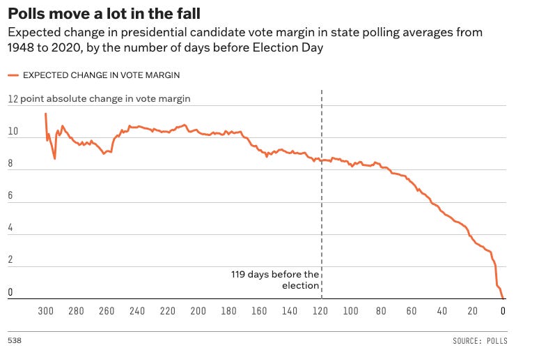
Assuming it isn’t Election Day, the model looks at how much polls have moved on average dependent on the number of days remaining to the election, and adds that value to the deviation too. (See the FiveThirtyEight chart below)
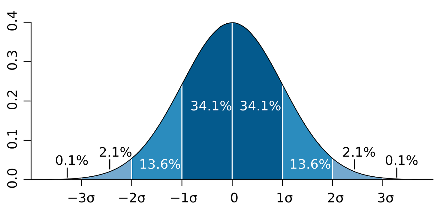
Now, the model will simulate the error itself, by taking the average historical error and applying the adjusted deviation within a normal random distribution, which means 0 on the chart below is the average error, and each point out from 0 is a distance of that adjusted deviation. This way, the vast majority (68%) of errors will fall within our given range, but some (32%) will be edge cases where there is an even larger error, to be extra cautious and uncertain.
An important distinction to make here is that the model is non-partisan when determining error, meaning that even if polls have significantly favored Democrats by 20 points historically, it will just assume that that state’s polling can be off 20 points either way. As such, the next step is to flip a coin and decide which party the error should favor. This is also where we simulate third-party error, which simply uses a uniform random distribution where the two ends are positive and negative of the Harris-Trump polling error. (in English, if there is a 5% polling error either way, the third-party share could be either boosted or lowered by 5%)
Now we can finally take all the adjusted-for-error vote shares and standardize them to equal 100% together, getting the final state result in that simulation. Next, those percentages are applied to turnout estimates from ElectionPredictionsOfficial.com, which seems to be the only publicly available turnout model. We now have an actual raw vote count for each state, all of which can be summed up to get our popular vote across the whole country, which is converted to the percentages that you see on the forecast page.
The model uses the percentages and state popular votes to determine who won the state, and then adds the electoral votes accordingly. As mentioned earlier, Maine and Nebraska complete this process for the two and three congressional districts (respectively) individually and add those districts up to get a statewide result.
We’re now getting into the final steps. The model repeats the process described above for all of the 56 (50 states, D.C., 5 congressional districts) jurisdictions in the election, and then checks to see who crossed the 270-electoral-vote threshold, or if there was a 269-269 tie. The number of simulations won by each candidate is divided by 100,000 to get the chance of winning for both. We also check for landslide wins (350+ electoral votes), determine the popular vote winner odds, the range of electoral outcomes w/ an 80% confidence interval, and the number of times there is an Electoral College/Popular vote split, like in 2016. Of course, we also track the individual state odds, which are shown on the forecast cartogram/map.
8. Post all the graphics, and finally go to bed.
That’s about it! I then run a few tools and copy over a few numbers to get the charts updated, and the forecast is up to date for the day. I hope to write more articles explaining more intricacies within the model later, and if you have any questions or ideas, or if I missed something here, feel free to comment on the article and let me know. If you’ve read all of this, I am impressed.


